We are really behind on our periodicals, and have quite the stack building up on our bookshelf. We’re going to be catching up over the next few days with a flurry of reading and posting.
[The] Quincy Institute for Responsible Statecraft, which states that its mission is to “move US foreign policy away from endless war and toward vigorous diplomacy in the pursuit of international peace.”
This think tank is apparently the love-child between a number of liberals and conservatives, including perennial boogeyman George Soros and arch-fiend David Koch. This is really promising. If The Quincy can be effective at keeping the US out of the next international conflict, then I am all for it.
One notable takeaway that I hadn’t heard before is Quincy’s executive director’s definition of transpartisanship, as opposed to bipartisanship. Bipartisanship, she explains, implies that each side is giving up some of what they want in compromise. Transpartisanship means that both sides are “collaborating on issues they already are in agreement over.” It’s a definition that I will be stealing in the future.
Marie Newmann vs. the Democratic Machine, by Rebecca Grant: If ever there was a subject near and dear and to me, it’s Progressive challengers to the Democratic party establishment. I’m not ready to dox myself quite yet, but I was an organizer for the 2016 Sanders campaign, as well as a staff for an unsuccessful Congressional primary campaign. This article does well to highlight Newmann’s challenge to conservative Democratic representative Dan Lipinkski, but I’m not sure there’s more to take away from it.
Right-Wing Troika, by Bryce Convert: Review of State Capture, by Alexander Hertel-Fernandez. State-level politics is another game that I’ve been involved with, and Republican Scott Walker’s successes in Wisconsin has been something that’s interested me. In my case, it’s been to pine that Democrats hadn’t dropped the ball so spectacularly over the past decade and lost so many state legislative seats and governors mansions. The GOP had a great strategy and implemented it brilliantly, with ALEC and other think tanks that helped push policy out in the states.
The left has a lot to learn from the conservative playbook, especially the Wisconsin model, and has a long ways to go to catch up. Hopefully State Capture will help the road to recovery.
In our previous posts (part 1, part 2) we showed how to get historical stock data from the Alpha Vantage API, use Pickle to cache it, and how prep it in Pandas. Now we are ready to throw it in Prophet!
So, after loading our main.py file, we get ticker data by passing the stock symbol to our get_symbol function, which will check the cache and get daily data going back as far as is available via AlphaVantage.
>>> symbol = "ARKK"
>>> ticker = get_symbol(symbol)
./cache/ARKK_2019_10_19.pickle not found
{'1. Information': 'Daily Prices (open, high, low, close) and Volumes', '2. Symbol': 'ARKK', '3. Last Refreshed': '2019-10-18', '4. Output Size': 'Full size', '5. Time Zone': 'US/Eastern'}
{'1: Symbol': 'ARKK', '2: Indicator': 'Simple Moving Average (SMA)', '3: Last Refreshed': '2019-10-18', '4: Interval': 'daily', '5: Time Period': 60, '6: Series Type': 'close', '7: Time Zone': 'US/Eastern'}
{'1: Symbol': 'ARKK', '2: Indicator': 'Relative Strength Index (RSI)', '3: Last Refreshed': '2019-10-18', '4: Interval': 'daily', '5: Time Period': 60, '6: Series Type': 'close', '7: Time Zone': 'US/Eastern Time'}
./cache/ARKK_2019_10_19.pickle saved
Running Prophet
Now we’re not going to do anything here with the original code other than wrap it in a function that we can call again later. Our alpha_df_to_prophet_df() function renames our datetime index and close price series data columns to the columns that Prophet expects. You can follow the original Medium post for an explanation of what’s going on; we just want the fitted history and forecast dataframes in our return statement.
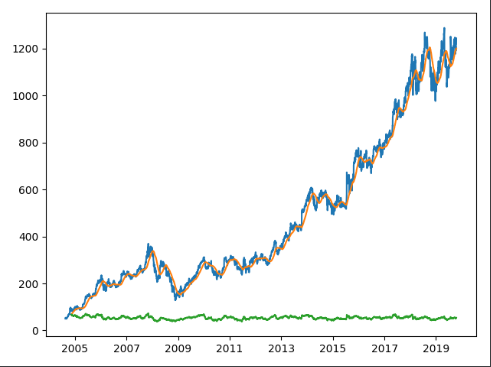
The whole process runs within a minute. Even twenty years of Google daily data can be processed quickly.
The last thing we want to do is concat the forecast data back to the original ticker data and Pickle it back to our file system. We rename our index back ‘date’ as it was before we modified it, then join it to the original Alpha Vantage data.
def concat(ticker, df_forecast):
    df = df_forecast.rename(columns={'ds': 'date'}).set_index('date')[['trend', 'yhat_lower', 'yhat_upper', 'yhat']]
    frames = [ticker, df]
    result = pd.concat(frames, axis=1)
    return result
Seeing the results
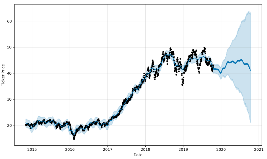
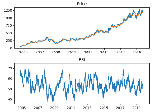
Since these are Pandas dataframes, we can use matplotlib to see the results, and Prophet also includes Plotly support. But as someone who looks at live charts in TradingView throughout the day, I’d like something more responsive. So we loaded the Bokeh library and created the following function to match.
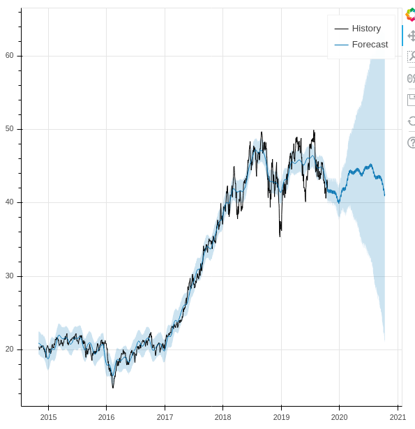
ARKK plot using matplotlib. Static only. ARKK plot in Plotly. Not great. UI is clunky and doesn’t work well in my dev VM browser.
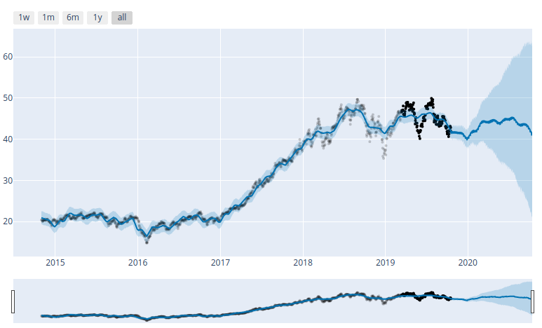
ARKK plot in Bokeh. Can easily zoom and pan. Lovely.
Putting it all together
Our ultimate goal here is to be able to process large batches of stocks, downloading the data from AV and processing it in Prophet in one go. For our initial run, we decided to start with the bundle of stocks in the ARK Innovation ETF. So we copied the holdings into a Python list, and created a couple of functions. One to process an individual stock, an another to process the list. Everything in the first function should be familiar except for two things. One, we added a check for the ‘yhat’ column to make sure that we didn’t inadvertently reprocess any individual stocks while we were debugging. We also refactored get_filename, which just adds the stock ticker plus today’s date to a string. It’s used in get_symbol during the Alpha Vantage call, as well as here when we save the Prophet-ized data back to the cache.
Finally, our process_list function. We had a bit of a wrinkle at first. Since we’re using the free AlphaVantage API, we’re limited to 5 API calls per minute. Now since we’re making three in each get_symbol() call we get an exception if we process the loop more than once in sixty seconds. Now I could have just gotten rid of the SMA and RSI calls, ultimately decided just to calculate the duration of each loop and just sleep until the minute was up. Obviously not the most elegant solution, but it works.
def process_list(symbol_list):
    for symbol in symbol_list:
        start = time.time()
        process(symbol)
        end = time.time()
        elapsed = end - start
        print ("Finished processing {} in {}".format(symbol, elapsed))
        if elapsed > 60:
            continue
        elif elapsed < 1:
            continue
        else:
            print('Waiting...')
            time.sleep(60 - elapsed)
            continue
So from there we just pass our list of ARKK stocks, go for a bio-break, and when we come back we’ve got a cache of Pickled Pandas data and Bokeh plots for about thirty stocks.
Where do we go now
Now I’m not putting too much faith into the results of the Prophet data, we didn’t do any customizations, and we just wanted to see what we can do with it. In the days since I started writing up this series, I’ve been thinking about ways to calculate the winners of the plots via a function call. So far I’ve come up with this discount function, that determines the discount of the current price of an asset relative to Prophet’s yhat prediction band.
A negative number for the discount indicates that the current price is below the prediction band, and may be a buy. Likewise, anything over 100 is above the prediction range and is overpriced, according to the model. We did ultimately pick two out of the ARKK holding that were well below the prediction range and showed a long term forecast, and we’ve started scaling in modestly while we see how things play out.
If we were more cautious, we’d do more backtesting, running limited time slices through Prophet and comparing forecast accuracy against the historical data. Additionally, we’d like to figure out a way to weigh our discount calculation against the accuracy projections.
There’s much more to to explore off of the original Medium post. We haven’t even gotten into integrating Alpha Vantage’s cryptoasset calls, nor have we done any of the validation and performance metrics that are part of the tutorial. It’s likely a part 4 and 5 of this series could follow. Ultimately though, our interest is to get into actual machine learning models such as TensorFlow and see what we can come up with there. While we understand the danger or placing too much weight into trained models, I do think that there may be value to using these frameworks as screeners. Coupled with the value averaging algorithm that we discussed here previously, we may have a good strategy for long-term investing. And anything that I can quantify and remove the emotional factor from is good as well.
I’ve learned so much doing this small project. I’m not sure how much more we’ll do with Prophet per se, but the Alpha Vantage API is very useful, and I’m guessing that I’ll be doing a lot more with Bokeh in the future. During the last week I’ve also discovered a new Python project that aims to provide a unified framework for coupling various equity and crypto exchange APIs with pluggable ML components, and use them to execute various trading strategies. Watch this space for discussion on that soon.
Facebook’s Prophet module is a trend forecasting library for Python. We spent some time over the last week going over it via this awesome introduction on Medium, but decided to do some refactoring to make it more reusable. Previously, we setup our pipenv virtual environment, separated sensitive data from our source code using dotenv, and started working with Alpha Vantage’s stock price and technical indicator API. In this post we’ll save our fetched data using Pickle and do some dataframe manipulations in Pandas. Part 3 is also available now.
Pickling our API results
When we left off, we had just wrote our get_time_series function, to which we pass 'get_daily' or such and a symbol for the stock that we would like to retrieve. We also have our get_technical function that we can use to pull any of the dozens of indicators available through Alpha Vantage’s API. Following the author’s original example, we can load Apple’s price history, simple moving average and RSI using the following calls:
symbol = 'AAPL'
ticker = get_time_series('get_daily', symbol, outputsize='full')
sma = get_technical('get_sma', symbol, time_period=60)
rsi = get_technical('get_rsi', symbol, time_period=60)
We’ve now got three dataframes. In the original piece, the author shows how you can export and import this dataframe using Panda’s .to_csv and read_csv functions. Saving the data is a good idea, especially during this stage of development, because it allows us to cache out data and reduce the number of API calls. (Alpha Vantage’s free tier allows 5 calls per minute, 500 a day. ) However, using CSV to save Panda’s dataframes is not recommended, as you will use index and column data. Python’s Pickle module will serialize the data and preserve it whole.
For our implementation, we will create a get_symbol function, which will check a local cache folder for a copy of the ticker data and load it. Our file naming convention uses the symbol string plus today’s date. Additionally, we concat our three dataframes into one using Pandas concat function:
def get_symbol(symbol):
    CACHE_DIR = './cache'
    # check if cache exists
    symbol = symbol.upper()
    today = datetime.now().strftime("%Y_%m_%d")

    file = CACHE_DIR + '/' + symbol + '_' + today + '.pickle'
    if os.path.isfile(file):
        # load pickle
        print("{} Found".format(file))
        result = pickle.load(open(file, "rb"))
    else:
        # get data, save to pickle
        print("{} not found".format(file))
        ticker = get_time_series('get_daily', symbol, outputsize='full')
        sma = get_technical('get_sma', symbol, time_period=60)
        rsi = get_technical('get_rsi', symbol, time_period=60)

        frames = [ticker, sma, rsi]
        result = pd.concat(frames, axis=1)
        pickle.dump(result, open(file, "wb"))
        print("{} saved".format(file))
    return result
Charts!
The original author left out all his chart code, so I had to figure things out on my own. No worries.
We saved both of these in a plot_ticker function for reuse in our library. Now I am no expert on matplotlib, and have only done some basic stuff with Plotly in the past. I’m probably spoiled by looking at TradingView’s wonderful chart tools and dynamic interface, so being able to drag and zoom around in the results is really important to me from a usability standpoint.
Now I am no expert on matplotlib, and have only done some basic stuff with Plotly in the past. I’m probably spoiled by looking at TradingView’s wonderful chart tools and dynamic interface, so being able to drag and zoom around in the results is really important to me from a usability standpoint. So we’ll leave matplotlib behind from here, and I’ll show you how I used Bokeh in the next part.
Framing our data
We already showed how we concat our price, SMA and RSI data together earlier. Let’s take a look at our dataframe metadata. I want to show you the columns, the dtype of those columns, as well as that of the index. Tail is included just for illustration.
>>> ticker.columns
Index(['1. open', '2. high', '3. low', '4. close', '5. volume', 'SMA', 'RSI'], dtype='object')

>>> ticker.dtypes
1. open      float64
2. high      float64
3. low       float64
4. close     float64
5. volume    float64
SMA          float64
RSI          float64
dtype: object

>>> ticker.index
DatetimeIndex(['1999-10-18', '1999-10-19', '1999-10-20', '1999-10-21',
               '1999-10-22', '1999-10-25', '1999-10-26', '1999-10-27',
               '1999-10-28', '1999-10-29',

>>> ticker.tail()
            1. open  2. high  3. low  4. close   5. volume       SMA      RSI
date
2019-10-09   227.03   227.79  225.64    227.03  18692600.0  212.0238  56.9637
2019-10-10   227.93   230.44  227.30    230.09  28253400.0  212.4695  57.8109
Now we don’t need all this for Prophet. In fact, it only looks at two series, a datetime column, labeled ‘ds’, and the series data that you want to forecast, a float, as ‘y’. In the original example, the author renames and recasts the data, but this is likely because of the metadata loss when importing from CSV, and isn’t strictly needed. Additionally, we’d like to preserve our original dataframe as we test our procedure code, so we’ll pass a copy.
In the first line of prophet_df =we’re selecting only the ‘close’ price column, which is returned with the original DateTimeIndex. We reset the index, which makes this into a ‘date’ column. Finally we rename them accordingly.
And that’s it for today! Next time we will be ready to take a look at Prophet. We’ll process our data, use Bokeh to display it, and finally write a procedure which we can use to process data in bulk.
I’ve spent countless hours this past week working with Facebook’s forecasting library, Prophet. I’ve seen lots of crypto and stock price forecasting and prediction model tutorials on Medium over the past few months, but this one by Senthil E. focusing on Apple and Bitcoin prices got my attention, and I just finished putting together a Python file that takes his code and builds it into some reusable code.
Now after getting to know it better, I can say that it’s not the most sophisticated package out there. I don’t think it was intended for forecasting stock data, but it is fast and allows one to see trends. Plus I learned a lot using it, and had fun. So what more can you ask for?
As background, I’ve been working on refining the Value Averaging functions I wrote about last week and had been having some issues with the Pandas Datareader library’s integration with the Alpha Vantage stock history API. Senthil uses a different third-party module that doesn’t have any problems, so that was good.
Getting started
I ran into some dependency hell during my initial setup. I spawned a new pipenv virtual environment and installed Jupyter notebook, but a prompt-toolkit conflict led to some wasted time. I started by copying the original code into a notebook, and go that running first. I quickly started running into problems with the author’s code.
I did get frustrated at one point and setup Anaconda in a Docker container on another machine, but I was able to get my main development machine up and running. We’ll save Conda for another day!
Importing the libraries
Like most data science projects, this one relies on Pandas and matplotlib, and the Prophet library has some Plotly integration. The author had the unused wordcloud package in his code for some reason as well, and it’s not entirely certain how he’s using the seaborn module, since he doesn’t explain his plots. He also listed two different Alpha Vantage modules despite only using one. I believe he may have put the alphaVantageAPI module in first before switching to the more useable alpha_vantage one.
We eventually added pickle, dotenv, and bokeh modules, as we’ll see shortly, as well as os, time, datetime.
import os
import pickle
import time
from datetime import datetime
import pandas as pd
from fbprophet import Prophet
from fbprophet.plot import plot_plotly
from bokeh.plotting import figure, output_file, show, save

import matplotlib.pyplot as plt
# import plotly.offline as py
# import numpy as np
# import seaborn as sns
# from alphaVantageAPI.alphavantage import AlphaVantage

from alpha_vantage.timeseries import TimeSeries
from alpha_vantage.techindicators import TechIndicators
from dotenv import load_dotenv
Protect your keys!
One of the first modules that we add to every project nowadays is python-dotenv. I’ve really been trying to get disciplined about 12-factor applications, and since I’m committing all of my projects to Gitlab these days, I can be sure not to commit my API keys to a repo or post them in a gist on my blog!
Also, pipenv shell automatically loads .env files, which is another reason why you should be using them.
If there is anything I hate, it’s repeating myself, or having to use the same block of code several times within a document. Now I don’t know whether the author kept the following two blocks of code in his story for illustrative purposes, or if this is just how he had it loaded in his notebook, but it gave me a complex.
from alpha_vantage.techindicators import TechIndicators
import matplotlib.pyplot as plt
ti = TechIndicators(key='<YES, he left his API KEY here!>',output_format='pandas')
data, meta_data = ti.get_sma(symbol='AAPL',interval='daily', time_period=60,series_type = 'close')
data.plot()
plt.show()

from alpha_vantage.techindicators import TechIndicators
import matplotlib.pyplot as plt
ti = TechIndicators(key='Youraccesskey',output_format='pandas')
data, meta_data = ti.get_rsi(symbol='AAPL',interval='daily', time_period=60,series_type = 'close')
data.plot()
plt.show()
If you look at the Alpha Vantage API documentation, there are separate endpoints for the time series and technical endpoints. The time series endpoint has different function calls for daily, weekly, monthly, &c.., and the Python module we’re using has separate methods for each. Same for the technical indicators. Now in the past, when I’ve tried to wrap APIs I would have had separate calls for each function, but I learned something about encapsulation lately and wanted to give something different a try.
Since the technical indicators functions share the same set of positional arguments, we can create a wrapper function where we pass the the name of the function (the indicator itself) that we want to get, the associated symbol, as well as any keyword arguments that we want to specify. We use the getattr method to find the class’s function by name, and pass on our variables using **kwargs.
def get_technical(indicator, symbol, **kwargs):
    function = getattr(ti, indicator)
    data, meta_data = function(symbol=symbol, **kwargs)
    print(meta_data)
    return data

sma = get_technical('get_sma', symbol, time_period=60)
rsi = get_technical('get_rsi', symbol, time_period=60)
Since most of the kwargs in the original were redundant, we only need to pass what we want to override. We’ve not really reduced the original code, to be honest, but we can customize what happens after in a way that we can be consistent, without having to write multiple functions for each function in the original module. Additionally, we can do this for the time series functions as well.
# BEFORE
from alpha_vantage.timeseries import TimeSeries
import matplotlib.pyplot as plt
ts = TimeSeries(key='Your Access Key',output_format='pandas')
apple, meta_data = ts.get_daily(symbol='AAPL',outputsize='full')
apple.head()

#AFTER
def get_time_series(time_series, symbol, **kwargs):
    function = getattr(ts, time_series)
    data, meta_data = function(symbol=symbol, **kwargs)
    print(meta_data)
    return data

ticker = get_time_series('get_daily', symbol, outputsize='full')
You can see that both functions are almost identical, except that the getattr call is passing the ts and ti classes. Ultimately, I’ll extend this to the cryptocurrencies endpoint as well, and be able to add any exception checking and debugging that I need for the entire module, and use one function for all of it.
Writing this code was one of those level-up moments when I got an idea and knew that I ultimately understood programming at an entirely different level than I had a few months ago.
Next, we’ll use Pickle to save and load our data, and start manipulating our dataframes before passing them to Prophet. Read part two.
I completed my three day fast last Thursday, and, as I recall from last time, the third day was much easier than the second. My main mistake was not carrying a huge bottle of water around with me the entire time. I drank tea several times during the first two days and it made me feel better each time, but I think the issue may have just been dehydration in general. Having something in the belly to keep the stomach from grumbling helped as well.
In general, I believe that I was in much worse condition when I started this fast. I’ve been drinking a lot of sugary drinks lately, and was probably closer to ketosis that I have been recently, so the problems I had those first two days were likely accountable to that factor.
Breaking my fast in the evening this time seems like it may have been a better for me in some respects, but I think I may try to time it for breakfast the next fast since it’s probably easier to finish the last few hours while sleeping instead of going the entire day and trying to kill those last few hours while preparing for the first meal in three days. In my case it was Pad Thai, dumplings and rolls, followed by everything I could get my hands on for the following hours. I’ve been scaling back into my time-restricted fasting schedule, and am going back on my regular 11AM-8PM schedule starting now.
100 days alcohol-free
Thursday was also 100 days alcohol-free for me, which is probably something that hasn’t happened since I was a teenager. I don’t know if this means I’m a teetotaler now or what. At this point it’s not about drinking so much as it is about spending my money on alcohol. It’s not like I threw out my liquor and wine — I still have a couple unopened bottles sitting on the hutch that I’m saving, but at this point the habit of not drinking has its own momentum. And although I haven’t thought about it too much, being on caffeine and staying up late working on code or whatever is a much better feeling the next morning than staying up drinking.
So we are almost 44 hours through our 72 hour fast, or about 60% of the way. I’ve been struggling a bit today, but I don’t think I’m feeling as bad as I did yesterday. I was very cranky and weak yesterday, but I don’t know how much of that was just due to the weather and the fact that my kids were being extremely obnoxious.
One thing weird happened this morning to me that is worth noting. When I was in the shower this morning and closed my eyes, I saw an afterimage. I stared at it, still with my eyes closed, and it took on a very distinctive shape, and became very vivid. But the strangest thing about it was that it retained its position in space as I moved my eyes around. Normally, when looking at an afterimage in physical space, it seems to move as the eyes move, but this did not. And the pure distinctiveness of the image was very remarkable. I could see it and look at it. I opened my eyes and closed them a few times to see what happened, and the effect persisted for some time.
Other than that, I’ve been trying to keep my belly full with water. I had a couple energy drinks yesterday, which was a mistake; I had some heart pounding after the second one yesterday afternoon. Today I just had tea and coffee and things seem OK. Heart pounding after getting up or going up stairs seems to be similar to what I experienced last time. I had 500mg of melanin before bed last night and slept well, I’ll do the same tonight.
I don’t remember how I managed to do this last time with the kids around. I think I may have done it during the weekend. Part of my crankiness last night was due to the fact that my kids wouldn’t stay at the table and kept getting up or trying to bring food into the living room, which they know is against the rules. I understand why Dr. Peter Attia doesn’t like to fast around his kids. Nothing is more annoying than a small child crying that they’re starving less than two hours after you’ve served them dinner.
So today marks the start of my second three-day fast. I scheduled this one right after I finished the first one, about three months ago, and I must say I’m a bit more nervous about this one than I was the first time. I think it’s probably because I feel like I’m a bit unprepared. I’ve been consuming a lot of caffeine and sugar lately, and I think I was a lot closer to a keto-friendly diet the first time I did this. We’ll see how things go.
I signed on a new client today. This one is a new landscaping company that my wife hired a couple weeks ago to do our yard. I’ll be setting up web and digital presence for them, putting together a branding and online marketing package. The other part of this will be helping them setup the operational tools as well. I think we’re going to do Jobber as it seems like the most features that they need: CRM, quoting, job management and invoicing. Pretty much the entire job lifecycle. Should be fun.
It also looks like I’ll be moving forward with setting up a Shopify site. I’ll probably try to sub this out, but we’ll see how much I think I can do on that.
I went ahead and pulled the trigger on Basecamp. It seems like the best of all the other project and client management software that I’ve seen. I’ll probably wind up having to pull Harvest into my stack as well just for timekeeping. The only other thing I’m missing is accounting. Right now I’m sending invoices through Paypal, but I’m going to need something more full featured. I know I don’t want Quickbooks. Freshbooks and Xero are the only two that I’m really aware of at the moment, so I’ll have to find something to use. Between the wife and I, we’re starting to take on a lot of additional work that will need tracking. I’ve been able to handle our tax returns via Turbotax Self Employed, but I don’t think it’s going to cut it much longer.
I spent most of the day hunched at my laptop, checking out git branches trying to rebase commits to clean up the project I’m working on, but I haven’t been having much success. I did, have some good progress with automated documentation and code review tools, as well as some Docker stuff.
I found an interesting presentation by a dev named Uilian Ries titled Creating C++ applications with Gitlab CI, which is exactly what I’m hoping to do. He mentions tools such as Cppcheck, Clang Tidy, and Doxygen. Now I remember something about automated documentation generators during one of my CS classes a couple semesters ago, but let me say that I really should have paid more attention.
Code dependencies for a wallet address creation test class in the Cryptonote codebase. Generated by the Doxygen automated documentation tool.
Uilian goes into a lot more during his presentation that I didn’t get into today, but I did start to work on automating the build process using Docker. One of the problems that I’ve run into with the original Cryptonote forks is that it was built for Ubuntu 16, using an older version of the Boost library. I haven’t quite figured out how to get the builds to work on Ubuntu 18, and keeping an older distro running somewhere isn’t really an effective use of time. I already had Docker setup on a home server, so I was able to spin a copy up, clone my repo, install build prereqs and go to town.
docker run --name pk_redux -it ubuntu:16.04
root@5a1d66905643:/#
apt-get update
apt-get install git
git clone https://gitlab.com/pk_redux/pkcli.git
cd pkcli
apt install screen make cmake build-essential libboost-all-dev pkg-config libssl-dev libzmq3-dev libunbound-dev libsodium-dev libminiupnpc-dev libreadline6-dev libldns-dev
make
.build/release/src/pkdaemon
My next step here is to save these commands into a Dockerfile or docker-compose file that I can start building off of, adding the code checks and documentation generators as needed. Once I’ve verified the syntax and worked out any bugs, I should be able to start adding things to the Gitlab CI YML files as well. This should help keep the project well-maintained and clean.
I’ve been familiar with Docker for some time, but it’s been a long time since I last messed around with it. It’s really exciting, to be able to document everything, and be able to spin up containers without polluting my base system.
I have been trying to get a grip on the Pennykoin CLI code base for some time. One of the problems that I’ve had is that the original developer had a lot of false starts and stops, and there’s a lot of orphan branches like this:
Taken with GitKraken
If that wasn’t bad enough, at some point they decided to push the current code to a new repo, and lost the entire starting commit history. Whether this was intentional or not, I can’t say. It’s made it very tricky for me to backtrack through the history of the code and figure out where bugs were introduced. So problem number one that I’m dealing with is how to link these two repos together so that I have a complete history to search through.
Merging two branches
So we had two repos, which we’ll call pk_old and pk_new. I originally tried methods where I tried to merge the repos together using branches, but I either wound up with the old repo as the last commit, or with the new repo and none of the old history. I spent a lot of time going over my bash history file and playing with using my local directories as remote sources, deleting and starting over. Then I was able to find out that there was indeed a common commit between these two repos, and that all I had to do was add the old remote with the –tags option to pull in everything.
Now, I probably could have gotten away by just cloning the pk_new repo instead of initializing an empty directory and adding the remote, but we the end result should be the same. A quick check of the tags between the two original repos and my new one showed that everything was there.
The link between the two repos
Phantom branches
One of the things that we have to do as part of our pk_redux, as we’re calling it, is setup new repos that we actually have control over. This time around, everything will be setup properly as part of governance, so that I’m not the only one with keys to the kingdom in case I go missing. I want to take advantage of GitLab’s integrated CI/CD, as we’ve talked about before, so I setup a new group and pkcli repo. I pushed the code base up, and saw all the tags, but none of the branches were there.
The issue ultimately comes down to the fact that git branches are just pointers to a specific commit in a repository’s history. Git will pull the commits down from a remote as part of a fetch job, but not the pointers to those branches unless I physically checked them out. Only after I created these tracking branches on my local repo could I then push them to the new remote origin.
Fixing Pennykoin
So now that I’ve got a handle on this repo, my next step is to hunt some bugs. I’ll probably have to do some more work to try and de-orphan some of these early commits in the repo history, cause that will be instrumental in tracking down changes to the Cryptonote parameters. These changes are likely the cause for the boostrap issue that exists. And my other priority is figuring out if we can unlock the bugged coins. From there I’d like to implement a test suite, and make sure that there is are proper branching workflows for code changes.
Knowing when to sell is one of the problems I struggle with as a trader, both in equities and crypto markets. In the past, I’ve relied on what the Motley Fool has referred to as a ‘buy and hold forever’ strategy, and it’s worked out well for me with some of the bigger tech stocks. As someone who’s been focusing more on shorter time frames lately, I’ve been having less success. And after watching my crypto portfolio break six figures in the winter of 2017 before crashing almost ninety percent, I’ve been trying to find a way to ensure that I’m able to actually take some profits when my positions start taking those parabolic runs.
One of the interesting metrics around the USD price of Bitcoin is the Mayer Multiple, which is the multiple of the current BTC price over the 200-day moving average. Trace Mayer determined that, historically speaking, the best long-term strategy was to accumulate BTC when when the Mayer Multiple was under 2.4. For comparison, the last time we hit that level was late June of this year when BTC hit $14K. Now I have traditionally been one to dollar-cost average into BTC, weekly, but I had to stop my contributions for a variety of market and personal reasons, but one plan I have been thinking about is to sell a large share of my position when the MM hits 2.88. This is a number I cam up with just by looking at the charts, and is currently about $26,200.
So I was really interested by this strategy put together by former BlackRock portfolio manager Vishal Karir, on how to take profits before the next bitcoin recession. I’m not going to rehash the entire piece here, suffice to say it sets a static accumulation target, buys when the asset value is below this target, and sells when it’s above it. I wanted to do some backtesting with some of my assets and see what I came up with. So I wrote up the following code in a Google Collab doc so I could start playing around with it.
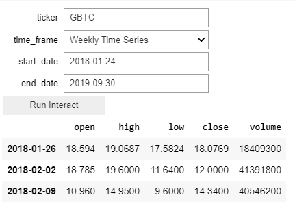
Instead of looking at BTC directly, I wanted to start by looking at the Grayscale BTC ETF, GBTC, so for this block we’re using Pandas wonderful datareader to pull quotes from AlphaVantage.
import os
from datetime import datetime
import pandas_datareader.data as web

!pip install ipywidgets
import ipywidgets as widgets
from ipywidgets import interact, interact_manual

os.environ['ALPHAVANTAGE_API_KEY'] = 'my_key'

f = ""

time_series = [
    ("Intraday Time Series", "av-intraday"),
    ("Daily Time Series", "av-daily"),
    ("Daily Time Series (Adjusted)", "av-daily-adjusted"),
    ("Weekly Time Series", "av-weekly"),
    ("Weekly Time Series (Adjusted)", "av-weekly-adjusted"),
    ("Monthly Time Series", "av-monthly"),
    ("Monthly Time Series (Adjusted)", "av-monthly-adjusted")
]


def get_asset_data (ticker, time_frame="av-weekly", start_date="2017-01-01", end_date="2019-09-30"):
  global f
  f = web.DataReader(ticker,
                     time_frame,
                     start = parse(start_date),
                     end = parse(end_date))
  return f

interact_manual(get_asset_data, ticker="", time_frame=time_series)
We’re using f as a global for our dataframe. It stores the stock data. We’re also using ipywidgets to allow us to easily change parameters for the data we want to run against.
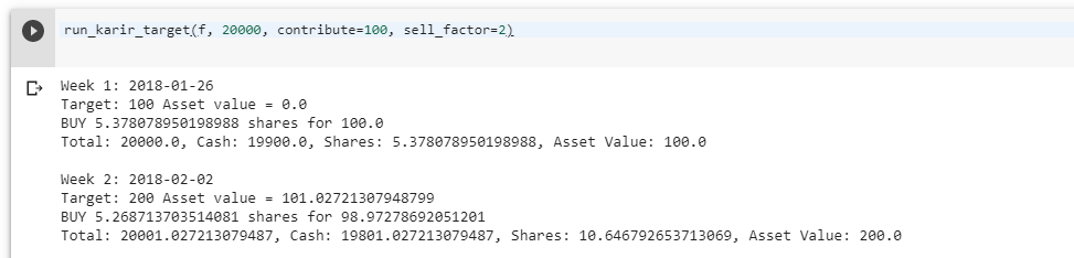
The next cell allows us to pass this previous dataframe to our backtest function. I wanted to play with various parameters such as the amount of capital available, the max contribution, and the ratio of max contributions to max sell amount.
Now there’s a lot here I will do later to clean up this code, making the params available via a widget as I did for the first function, but for now it works just fine. Here’s a test run with $100 contributed weekly from just after the beginning of the BTC bear market till now.
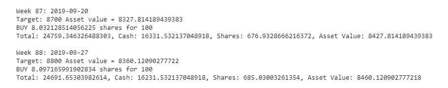
Week 1 and 2 of our backtestThe ‘bottom’.We’re not including the entire run, but here’s where we end up.
So, not bad on our hypothetical run. That’s a gain of almost $4700 off of $3769 invested, or a 24% return. Now we’re cherry-picking, or course. At the bottom of the market, we would have had over $7K deployed at a break even. But Karir’s strategy opens up a whole slew of possibilities, and what may be a good rule of thumb for scaling out of positions. Since I’ve been able to get this package working, I’ve been looking at other investments that I’ve made in equities markets, and am starting to form some hypotheses that may help guide best practices for both entries and exits.
My next step, after cleaning up this code a bit, is to figure out a way to run some regression tests on the sell multiple. I think a dynamic variable may actually be more helpful in instances where the asset goes on a parabolic run. But the point here is that I have a framework that I can test my assumptions against.
It shouldn’t be too hard also to integrate Karir’s strategy for accumulation of BTC, as well as altcoin pairings as well. It’s an exciting strategy for investment, and one that can be automated via exchange and broker APIs. There may also be some variations that we can deploy, using this kind of targeted portfolio value as a way to layer limit orders. For this simulation we simply used the open price of the time period, but we could calculate the price an asset would have to be for us to sell it next week, and set some orders in the present period. If the high for that period hits that level, we could simulate the trade and see how that affects our gains.