After publishing last night’s post, I made a little headway with one of my projects, figuring out how to mount a SQL dump into a mySQL Docker image so that it gets loaded automatically when the container spins up. Just one more little win toward accomplishing my task. Now I just need to tackle the way I have WordPress deployed, and I can begin working on the project for real. I’m taking my time with this. All of the learning and research I’m doing now isn’t the client’s time, it’s mine, and is the kind of learning I love.
Being able to master Docker means I don’t have to run all this stuff on my local machines. I can start culling all of the packages that I’ve loaded in the past for this project or that, things like Node dependencies, Ruby, and Postgres no longer have to bulk up my system. Pop, here’s a container. Pop, there it goes. I went through my staging server a few days ago and started cleaning out shop, removing abandoned projects. Goodbye, rm *pennykoin* -rf, and so long.
I’m still reading Fluent Python, about a half hour before bed. I finally have a good grasp on decorators. I think my eyes glazed over on coroutines, but I think I’m ready to add threading to my value averager app. I’ve only got a couple of chapters left, on asyncio, which I desperately need to master, and another on one of my favorite subjects, metaprogramming.
I’ve been reading Fluent Python for about twenty minutes right when I climb in the bed. It’s on the iPad and even with the brightness turned down all the way, it’s still bad for rest, so I usually wind up reading a real book. Right now it’s Digital Minimalism and last night there was a section about Henry David Thoreau, starting with his time building his cabin at Walden Pond, before he wrote his book. Just how does one build a cabin using just an axe? Anyways, the point here, and one I never knew before is that Walden is really about using time as the true unit of account. What use is earning a bunch more money if the cost in time to earn it is so much. And for what?
It’s not that I haven’t heard the idea of time as money before, or rather trading time for money. It’s very prevalent in the things I read and hear. Just realizing that Thoreau was writing about it some one hundred and fifty years ago makes me realize how little things have changed. I don’t know why I should be surprised. I’m sure Marcus Aurelius says similar things in his diaries. I think my point is that I wasn’t expecting to hear it. Here I was, trying to convince myself that I should delete Twitter off my phone for a month, and here’s Cal Newport, via Thoreau, asking “why are you working so hard, you sap?”
Thoreau did have any children, though, so I guess I can say that’s part of the reason that I grind, although it’s really not the only reason. I like figuring things out, and it’s just so happened that the things I’ve figured out how to do enables me to earn a comfortable living. Still, there’s some sort of drive to build something, a legacy, if you will, coupled with a mild regret that I should have more to show for this life I’ve lived these past forty one years. One of my grandfathers built a house. All I have of another is a stained glass lamp, sitting next to one of my daughter’s beds. That and memories of model trains in a basement, and playing a flight simulator on an old Tandy PC back in the 80’s.
And maybe that later point is the crux of minimalism. In the end, it is the memories that matter. Not all of us are going to write lasting works of fiction or build cathedrals that will be finished long after our deaths and stand for centuries. Today, all I can do is love those around me, and tinker on my keyboard, changing the world around me, bit by bit. Who knows, maybe Bitcoin is going to succeed, allowing me to leave generational wealth for my grandkids, either directly or indirectly. Maybe one of my other projects will succeed and grant me a minimum viable income so that I’m not forced to work another day in my life.
Maybe I’m being fatalistic, maybe this is just my monkey mind sowing doubt in my mind, preparing me for failure. I’m not sure, but it doesn’t feel like it. I think it’s just recognition that I’ve got too many things distracting me, things that I need to let go of, and remove from my life.
But right now, I hear the pitter patter of little feet upstairs, which means it’s time for me to enjoy my Sunday.
I spent most of the winter break working on automating a value averaging algorithm that I wrote about several months ago. Back in October we started scaling into three positions that we identified based on our work with some predictions we did using Facebook’s Prophet earlier. My goal was to develop a protocol and work out any kinks in the process manually while I worked on building out code that would eventually take over. While I’m not ready to release the modules to the public yet, I have managed to get the general order calculation and order placement up and running.
To start, I setup a Google Sheet with the details of each position: start date, number of days to run, and the total amount to invest. I used Alexander Elder’s Two Percent Rule, as usual to come up with this number. Essentially each position would be small enough that I wouldn’t need to setup stop losses. From there, the sheet would keep track of the number of business days (as a proxy for trading days) and would compute the target position size for that day. I would update a cell with the current instrument price, and the sheet would compute whether my asset holding was above or below the target, and calculate the buy or sell quantities accordingly.
After market open, I would update the price for each stock and put in the orders for each position. This took a few minutes each day, and became part of my morning routine over the past two months or so. Ideally, this process should have only taken five minutes out of my day, but we ran into some challenges due to the decisions we made that required us to rework things and audit our order history several times.
The first of these was based around the type of orders we placed. I decided that I didn’t want to market buy everything, and instead put ‘good-until-cancelled’ limit orders in. When there was no spread between the bid and the ask, I would just match whichever end I was on, and if there was a split I would put my order price one penny in the spread. As a result, some orders would go unfilled, and required some overly complicated spreadsheet calculations to keep track of which orders were filled, what my actual number of shares was ‘supposed’ to be, and so on. I also started using a prorated target, based on the number of days with actual filled orders. This became a problem to track. Also, some days there were large spreads, and my buy orders were way lower than anything that would get filled. There were times when the price fell for a few days and picked up some of these, but keeping track of these filled/unfilled orders was a huge pain in the butt.
One of the reasons that it took me so long to develop a working product was due to the challenges I had with existing Python support for my brokerage. The only feasible module that I could find on Pypi had basic functionality and required a lot of work. It had no order-placing capabilities, so I had to write those. I also got lost working through Ameritrade’s non-compliant schema definitions, and I almost gave up hope entirely when I found out that they were getting bought out. The module still has a lot of improvements needed before it can be run in a completely automated manner, but more on that later.
So far I’ve got just under a thousand lines of code — not as many tests as I should have written — that allows me to process a list of positions, tuples with stock ticker, days to run, start date, and total capital to invest. It calculates the ideal target, gets the current value of the position, and then calculates the difference and number of shares to buy or sell. It then places the order. I’m still manually keeping an eye on things and tracking my orders in the sheet as I’ve been doing, but there’s too much of a discrepancy between the Python algorithm and my spreadsheet. I don’t anticipate trying to wade through my transaction history to try to program around all of the mistakes and adjustments that I made during the development process. I’ll just have to live without the prorated targets for the time being.
I think priorities for the next few commits will be improving the brokerage module. Right now it requires Chromedriver to generate the authentication tokens; this can be done using straight up request sessions. There’s also no error checking; session expiration is a common problem and I had to write a function to use to refresh it without reauthentication. So first priority will be getting the the order placement calls and token handling improvements put in and a PR back into the main module.
From there, I’d like to clean up the Quicktype-generated objects and get them moved over to the brokerage package where they belong. I don’t know that most people are going to want to use Python objects instead or dictionaries, but I put enough work into it that I want it out there.
Lastly, I’ll need to figure out how to separate any of the broker-specific function calls from the value averaging functions. Right now it’s too intertwined to be used for anything other than my brokerage, so I’ll see about getting it generalized in such a way that it can be used with Tensortrade or other algorithmic trading platforms.
I’m not sure how much of this I can get done over the spring. Classes for my final semester at school start next Monday, and it will be May before I’m done with classes. But I will keep posting updates.
In our previous posts (part 1, part 2) we showed how to get historical stock data from the Alpha Vantage API, use Pickle to cache it, and how prep it in Pandas. Now we are ready to throw it in Prophet!
So, after loading our main.py file, we get ticker data by passing the stock symbol to our get_symbol function, which will check the cache and get daily data going back as far as is available via AlphaVantage.
>>> symbol = "ARKK"
>>> ticker = get_symbol(symbol)
./cache/ARKK_2019_10_19.pickle not found
{'1. Information': 'Daily Prices (open, high, low, close) and Volumes', '2. Symbol': 'ARKK', '3. Last Refreshed': '2019-10-18', '4. Output Size': 'Full size', '5. Time Zone': 'US/Eastern'}
{'1: Symbol': 'ARKK', '2: Indicator': 'Simple Moving Average (SMA)', '3: Last Refreshed': '2019-10-18', '4: Interval': 'daily', '5: Time Period': 60, '6: Series Type': 'close', '7: Time Zone': 'US/Eastern'}
{'1: Symbol': 'ARKK', '2: Indicator': 'Relative Strength Index (RSI)', '3: Last Refreshed': '2019-10-18', '4: Interval': 'daily', '5: Time Period': 60, '6: Series Type': 'close', '7: Time Zone': 'US/Eastern Time'}
./cache/ARKK_2019_10_19.pickle saved
Running Prophet
Now we’re not going to do anything here with the original code other than wrap it in a function that we can call again later. Our alpha_df_to_prophet_df() function renames our datetime index and close price series data columns to the columns that Prophet expects. You can follow the original Medium post for an explanation of what’s going on; we just want the fitted history and forecast dataframes in our return statement.
The whole process runs within a minute. Even twenty years of Google daily data can be processed quickly.
The last thing we want to do is concat the forecast data back to the original ticker data and Pickle it back to our file system. We rename our index back ‘date’ as it was before we modified it, then join it to the original Alpha Vantage data.
def concat(ticker, df_forecast):
    df = df_forecast.rename(columns={'ds': 'date'}).set_index('date')[['trend', 'yhat_lower', 'yhat_upper', 'yhat']]
    frames = [ticker, df]
    result = pd.concat(frames, axis=1)
    return result
Seeing the results
Since these are Pandas dataframes, we can use matplotlib to see the results, and Prophet also includes Plotly support. But as someone who looks at live charts in TradingView throughout the day, I’d like something more responsive. So we loaded the Bokeh library and created the following function to match.
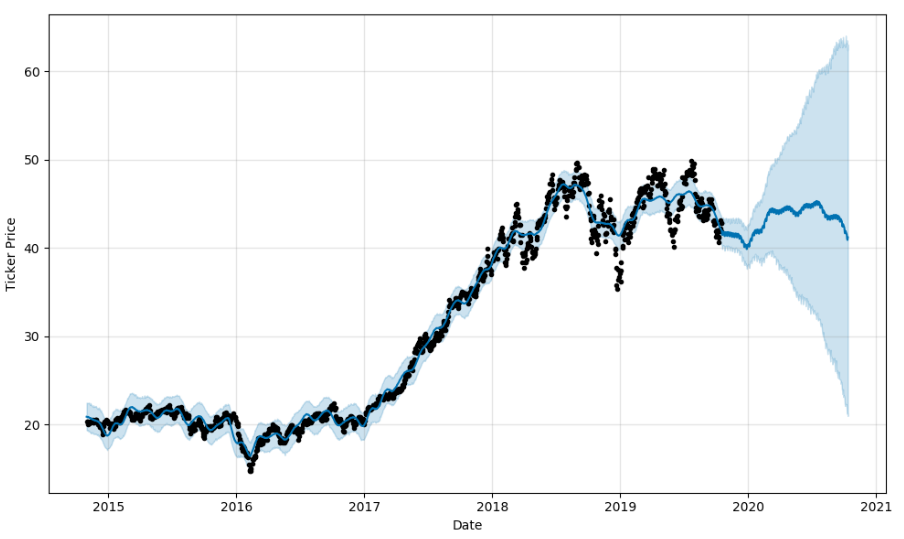
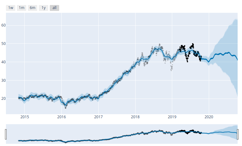
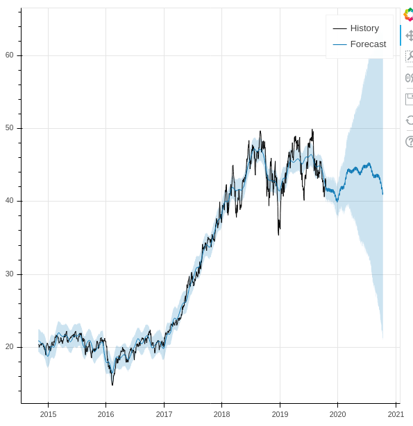
ARKK plot using matplotlib. Static only. ARKK plot in Plotly. Not great. UI is clunky and doesn’t work well in my dev VM browser.
ARKK plot in Bokeh. Can easily zoom and pan. Lovely.
Putting it all together
Our ultimate goal here is to be able to process large batches of stocks, downloading the data from AV and processing it in Prophet in one go. For our initial run, we decided to start with the bundle of stocks in the ARK Innovation ETF. So we copied the holdings into a Python list, and created a couple of functions. One to process an individual stock, an another to process the list. Everything in the first function should be familiar except for two things. One, we added a check for the ‘yhat’ column to make sure that we didn’t inadvertently reprocess any individual stocks while we were debugging. We also refactored get_filename, which just adds the stock ticker plus today’s date to a string. It’s used in get_symbol during the Alpha Vantage call, as well as here when we save the Prophet-ized data back to the cache.
Finally, our process_list function. We had a bit of a wrinkle at first. Since we’re using the free AlphaVantage API, we’re limited to 5 API calls per minute. Now since we’re making three in each get_symbol() call we get an exception if we process the loop more than once in sixty seconds. Now I could have just gotten rid of the SMA and RSI calls, ultimately decided just to calculate the duration of each loop and just sleep until the minute was up. Obviously not the most elegant solution, but it works.
def process_list(symbol_list):
    for symbol in symbol_list:
        start = time.time()
        process(symbol)
        end = time.time()
        elapsed = end - start
        print ("Finished processing {} in {}".format(symbol, elapsed))
        if elapsed > 60:
            continue
        elif elapsed < 1:
            continue
        else:
            print('Waiting...')
            time.sleep(60 - elapsed)
            continue
So from there we just pass our list of ARKK stocks, go for a bio-break, and when we come back we’ve got a cache of Pickled Pandas data and Bokeh plots for about thirty stocks.
Where do we go now
Now I’m not putting too much faith into the results of the Prophet data, we didn’t do any customizations, and we just wanted to see what we can do with it. In the days since I started writing up this series, I’ve been thinking about ways to calculate the winners of the plots via a function call. So far I’ve come up with this discount function, that determines the discount of the current price of an asset relative to Prophet’s yhat prediction band.
A negative number for the discount indicates that the current price is below the prediction band, and may be a buy. Likewise, anything over 100 is above the prediction range and is overpriced, according to the model. We did ultimately pick two out of the ARKK holding that were well below the prediction range and showed a long term forecast, and we’ve started scaling in modestly while we see how things play out.
If we were more cautious, we’d do more backtesting, running limited time slices through Prophet and comparing forecast accuracy against the historical data. Additionally, we’d like to figure out a way to weigh our discount calculation against the accuracy projections.
There’s much more to to explore off of the original Medium post. We haven’t even gotten into integrating Alpha Vantage’s cryptoasset calls, nor have we done any of the validation and performance metrics that are part of the tutorial. It’s likely a part 4 and 5 of this series could follow. Ultimately though, our interest is to get into actual machine learning models such as TensorFlow and see what we can come up with there. While we understand the danger or placing too much weight into trained models, I do think that there may be value to using these frameworks as screeners. Coupled with the value averaging algorithm that we discussed here previously, we may have a good strategy for long-term investing. And anything that I can quantify and remove the emotional factor from is good as well.
I’ve learned so much doing this small project. I’m not sure how much more we’ll do with Prophet per se, but the Alpha Vantage API is very useful, and I’m guessing that I’ll be doing a lot more with Bokeh in the future. During the last week I’ve also discovered a new Python project that aims to provide a unified framework for coupling various equity and crypto exchange APIs with pluggable ML components, and use them to execute various trading strategies. Watch this space for discussion on that soon.
Facebook’s Prophet module is a trend forecasting library for Python. We spent some time over the last week going over it via this awesome introduction on Medium, but decided to do some refactoring to make it more reusable. Previously, we setup our pipenv virtual environment, separated sensitive data from our source code using dotenv, and started working with Alpha Vantage’s stock price and technical indicator API. In this post we’ll save our fetched data using Pickle and do some dataframe manipulations in Pandas. Part 3 is also available now.
Pickling our API results
When we left off, we had just wrote our get_time_series function, to which we pass 'get_daily' or such and a symbol for the stock that we would like to retrieve. We also have our get_technical function that we can use to pull any of the dozens of indicators available through Alpha Vantage’s API. Following the author’s original example, we can load Apple’s price history, simple moving average and RSI using the following calls:
symbol = 'AAPL'
ticker = get_time_series('get_daily', symbol, outputsize='full')
sma = get_technical('get_sma', symbol, time_period=60)
rsi = get_technical('get_rsi', symbol, time_period=60)
We’ve now got three dataframes. In the original piece, the author shows how you can export and import this dataframe using Panda’s .to_csv and read_csv functions. Saving the data is a good idea, especially during this stage of development, because it allows us to cache out data and reduce the number of API calls. (Alpha Vantage’s free tier allows 5 calls per minute, 500 a day. ) However, using CSV to save Panda’s dataframes is not recommended, as you will use index and column data. Python’s Pickle module will serialize the data and preserve it whole.
For our implementation, we will create a get_symbol function, which will check a local cache folder for a copy of the ticker data and load it. Our file naming convention uses the symbol string plus today’s date. Additionally, we concat our three dataframes into one using Pandas concat function:
def get_symbol(symbol):
    CACHE_DIR = './cache'
    # check if cache exists
    symbol = symbol.upper()
    today = datetime.now().strftime("%Y_%m_%d")

    file = CACHE_DIR + '/' + symbol + '_' + today + '.pickle'
    if os.path.isfile(file):
        # load pickle
        print("{} Found".format(file))
        result = pickle.load(open(file, "rb"))
    else:
        # get data, save to pickle
        print("{} not found".format(file))
        ticker = get_time_series('get_daily', symbol, outputsize='full')
        sma = get_technical('get_sma', symbol, time_period=60)
        rsi = get_technical('get_rsi', symbol, time_period=60)

        frames = [ticker, sma, rsi]
        result = pd.concat(frames, axis=1)
        pickle.dump(result, open(file, "wb"))
        print("{} saved".format(file))
    return result
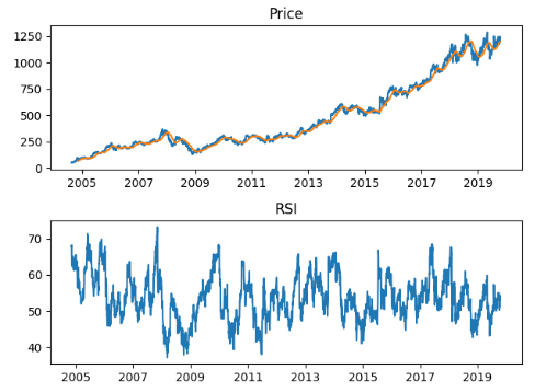
Charts!
The original author left out all his chart code, so I had to figure things out on my own. No worries.
We saved both of these in a plot_ticker function for reuse in our library. Now I am no expert on matplotlib, and have only done some basic stuff with Plotly in the past. I’m probably spoiled by looking at TradingView’s wonderful chart tools and dynamic interface, so being able to drag and zoom around in the results is really important to me from a usability standpoint.
Now I am no expert on matplotlib, and have only done some basic stuff with Plotly in the past. I’m probably spoiled by looking at TradingView’s wonderful chart tools and dynamic interface, so being able to drag and zoom around in the results is really important to me from a usability standpoint. So we’ll leave matplotlib behind from here, and I’ll show you how I used Bokeh in the next part.
Framing our data
We already showed how we concat our price, SMA and RSI data together earlier. Let’s take a look at our dataframe metadata. I want to show you the columns, the dtype of those columns, as well as that of the index. Tail is included just for illustration.
>>> ticker.columns
Index(['1. open', '2. high', '3. low', '4. close', '5. volume', 'SMA', 'RSI'], dtype='object')

>>> ticker.dtypes
1. open      float64
2. high      float64
3. low       float64
4. close     float64
5. volume    float64
SMA          float64
RSI          float64
dtype: object

>>> ticker.index
DatetimeIndex(['1999-10-18', '1999-10-19', '1999-10-20', '1999-10-21',
               '1999-10-22', '1999-10-25', '1999-10-26', '1999-10-27',
               '1999-10-28', '1999-10-29',

>>> ticker.tail()
            1. open  2. high  3. low  4. close   5. volume       SMA      RSI
date
2019-10-09   227.03   227.79  225.64    227.03  18692600.0  212.0238  56.9637
2019-10-10   227.93   230.44  227.30    230.09  28253400.0  212.4695  57.8109
Now we don’t need all this for Prophet. In fact, it only looks at two series, a datetime column, labeled ‘ds’, and the series data that you want to forecast, a float, as ‘y’. In the original example, the author renames and recasts the data, but this is likely because of the metadata loss when importing from CSV, and isn’t strictly needed. Additionally, we’d like to preserve our original dataframe as we test our procedure code, so we’ll pass a copy.
In the first line of prophet_df =we’re selecting only the ‘close’ price column, which is returned with the original DateTimeIndex. We reset the index, which makes this into a ‘date’ column. Finally we rename them accordingly.
And that’s it for today! Next time we will be ready to take a look at Prophet. We’ll process our data, use Bokeh to display it, and finally write a procedure which we can use to process data in bulk.
I’ve spent countless hours this past week working with Facebook’s forecasting library, Prophet. I’ve seen lots of crypto and stock price forecasting and prediction model tutorials on Medium over the past few months, but this one by Senthil E. focusing on Apple and Bitcoin prices got my attention, and I just finished putting together a Python file that takes his code and builds it into some reusable code.
Now after getting to know it better, I can say that it’s not the most sophisticated package out there. I don’t think it was intended for forecasting stock data, but it is fast and allows one to see trends. Plus I learned a lot using it, and had fun. So what more can you ask for?
As background, I’ve been working on refining the Value Averaging functions I wrote about last week and had been having some issues with the Pandas Datareader library’s integration with the Alpha Vantage stock history API. Senthil uses a different third-party module that doesn’t have any problems, so that was good.
Getting started
I ran into some dependency hell during my initial setup. I spawned a new pipenv virtual environment and installed Jupyter notebook, but a prompt-toolkit conflict led to some wasted time. I started by copying the original code into a notebook, and go that running first. I quickly started running into problems with the author’s code.
I did get frustrated at one point and setup Anaconda in a Docker container on another machine, but I was able to get my main development machine up and running. We’ll save Conda for another day!
Importing the libraries
Like most data science projects, this one relies on Pandas and matplotlib, and the Prophet library has some Plotly integration. The author had the unused wordcloud package in his code for some reason as well, and it’s not entirely certain how he’s using the seaborn module, since he doesn’t explain his plots. He also listed two different Alpha Vantage modules despite only using one. I believe he may have put the alphaVantageAPI module in first before switching to the more useable alpha_vantage one.
We eventually added pickle, dotenv, and bokeh modules, as we’ll see shortly, as well as os, time, datetime.
import os
import pickle
import time
from datetime import datetime
import pandas as pd
from fbprophet import Prophet
from fbprophet.plot import plot_plotly
from bokeh.plotting import figure, output_file, show, save

import matplotlib.pyplot as plt
# import plotly.offline as py
# import numpy as np
# import seaborn as sns
# from alphaVantageAPI.alphavantage import AlphaVantage

from alpha_vantage.timeseries import TimeSeries
from alpha_vantage.techindicators import TechIndicators
from dotenv import load_dotenv
Protect your keys!
One of the first modules that we add to every project nowadays is python-dotenv. I’ve really been trying to get disciplined about 12-factor applications, and since I’m committing all of my projects to Gitlab these days, I can be sure not to commit my API keys to a repo or post them in a gist on my blog!
Also, pipenv shell automatically loads .env files, which is another reason why you should be using them.
If there is anything I hate, it’s repeating myself, or having to use the same block of code several times within a document. Now I don’t know whether the author kept the following two blocks of code in his story for illustrative purposes, or if this is just how he had it loaded in his notebook, but it gave me a complex.
from alpha_vantage.techindicators import TechIndicators
import matplotlib.pyplot as plt
ti = TechIndicators(key='<YES, he left his API KEY here!>',output_format='pandas')
data, meta_data = ti.get_sma(symbol='AAPL',interval='daily', time_period=60,series_type = 'close')
data.plot()
plt.show()

from alpha_vantage.techindicators import TechIndicators
import matplotlib.pyplot as plt
ti = TechIndicators(key='Youraccesskey',output_format='pandas')
data, meta_data = ti.get_rsi(symbol='AAPL',interval='daily', time_period=60,series_type = 'close')
data.plot()
plt.show()
If you look at the Alpha Vantage API documentation, there are separate endpoints for the time series and technical endpoints. The time series endpoint has different function calls for daily, weekly, monthly, &c.., and the Python module we’re using has separate methods for each. Same for the technical indicators. Now in the past, when I’ve tried to wrap APIs I would have had separate calls for each function, but I learned something about encapsulation lately and wanted to give something different a try.
Since the technical indicators functions share the same set of positional arguments, we can create a wrapper function where we pass the the name of the function (the indicator itself) that we want to get, the associated symbol, as well as any keyword arguments that we want to specify. We use the getattr method to find the class’s function by name, and pass on our variables using **kwargs.
def get_technical(indicator, symbol, **kwargs):
    function = getattr(ti, indicator)
    data, meta_data = function(symbol=symbol, **kwargs)
    print(meta_data)
    return data

sma = get_technical('get_sma', symbol, time_period=60)
rsi = get_technical('get_rsi', symbol, time_period=60)
Since most of the kwargs in the original were redundant, we only need to pass what we want to override. We’ve not really reduced the original code, to be honest, but we can customize what happens after in a way that we can be consistent, without having to write multiple functions for each function in the original module. Additionally, we can do this for the time series functions as well.
# BEFORE
from alpha_vantage.timeseries import TimeSeries
import matplotlib.pyplot as plt
ts = TimeSeries(key='Your Access Key',output_format='pandas')
apple, meta_data = ts.get_daily(symbol='AAPL',outputsize='full')
apple.head()

#AFTER
def get_time_series(time_series, symbol, **kwargs):
    function = getattr(ts, time_series)
    data, meta_data = function(symbol=symbol, **kwargs)
    print(meta_data)
    return data

ticker = get_time_series('get_daily', symbol, outputsize='full')
You can see that both functions are almost identical, except that the getattr call is passing the ts and ti classes. Ultimately, I’ll extend this to the cryptocurrencies endpoint as well, and be able to add any exception checking and debugging that I need for the entire module, and use one function for all of it.
Writing this code was one of those level-up moments when I got an idea and knew that I ultimately understood programming at an entirely different level than I had a few months ago.
Next, we’ll use Pickle to save and load our data, and start manipulating our dataframes before passing them to Prophet. Read part two.