Grayscale Bitcoin Trust (GBTC) is the name of a publicly traded OTC investment product listed on the public OTC markets. It’s a way for US investors to take a position in Bitcoin through brokerage and retirement accounts like IRAs. A lot of OG crypto-types scoff at the prospect of purchasing such an asset, since you don’t actually control the BTC or the private keys, but for some this is an attractive option, or an only one. I’ve been personally taking positions in GBTC over the past 3 or so years through my retirement IRA. One of the most underlooked qualities of GBTC through an IRA is that all transactions are tax-free. I can take profits in my IRA at any time without worrying about tax liability, which is not something I can say for my actual crypto holdings.
Two of the downsides of GBTC is that Grayscale takes a two percent management fee. This isn’t a big deal to me because of the expected gains in a bull run. The other is that there is a premium on GBTC over the underlying asset value. Each share of GBTC represents .00096884 Bitcoin, but the GBTC’s price is usually 30-10% higher than the value of the underlying asset.
One of the main differences between the equities and crypto markets is the fact that crypto is 24/7. Often, during times when BTC has made a big price movement, I’ve wondered what the corresponding change in the price of GBTC would be (and in my portfolio!) So, I have written a small Python package to calculate this that I call GBTC Estimator.
I have it setup to get public BTC prices from Gemini (via the excellent CCXT package). Right now it’s using IEX’s daily GBTC data (and required an IEX API key), so it only has access to daily OHLCV (open, high, low, close, volume) data. We take the close price of GBTC, and divide it by the price of BTC at the same time (4PM EST) to come up with the actual BTC per share. This number is then used with the current BTC price to come up with the estimated GBTC value.
This current version is run from the command line and returns the estimated price as well as the difference from the last close in dollars and percentage. I have plans to put this up as a website that updates automatically, but first I think I’m going to do some backtesting to see how accurate this is. I think there may be some arbitrage opportunities to be found here. I’ve already started refactoring and will have more updates to follow.
Last night I had the pleasure of meeting Travis Oliphant, one of the primary creators of Numpy and and founder of Anaconda. He’s currently the CEO of OpenTeams, a company attempting to change the relationship between open source software and the companies that build on top of it. I found out about the lecture and was interested in it because of an article I had read in Wired about technology’s free rider problem, and went to the event without knowing anything much at all about Mr. Oliphant. I soon found out who he was and was very grateful that I had come. I’ve spent a lot of time using Numpy, and I’ll admit I was a bit starstruck.
Travis’s lecture spawned from his experience working on Numpy. He basically gave up tenure track at Brigham Young University to work on it, and had to find other ways to support his family for the two years that he was working on the initial release. As was noted elsewhere, much of the tech boom over the past 20 years has been built on top of the contributions of FOSS developers like Travis and others. He’s a big believer of profit, and thinks that the lack of financial incentives in the FOSS space has caused several problems, including developer to burnout, leading to a lack of proper maintenance of these projects. Many of these projects, like Numpy, have become crucially important to the scientific and business community.
Tim Oliphant’s Pycon 2019 Lighting Talk about Quansight
Oliphant’s goal is to make open source sustainable. Quansight is a venture fund for companies that rely on OSS, one of the ones they’ve funded is a public benefit corporation called FairOSS, which hopes to support OSS developers through contributions from companies that use OSS. He’s also doing something very similar with OpenTeams, hoping to follow Red Hat’s model of supporting Open Source by providing support contracts for various projects.
These are all very worthy goals, and I was both impressed and inspired by his talk. It’s opened up some interesting career opportunities. I recently took my first developer payment through GitCoin recently, and it was a bit of a rush. Getting paid to work on Open Source Software seems like an awesome opportunity, and I’ll be keeping an eye on this for potential post-graduate plans.
I spent most of the winter break working on automating a value averaging algorithm that I wrote about several months ago. Back in October we started scaling into three positions that we identified based on our work with some predictions we did using Facebook’s Prophet earlier. My goal was to develop a protocol and work out any kinks in the process manually while I worked on building out code that would eventually take over. While I’m not ready to release the modules to the public yet, I have managed to get the general order calculation and order placement up and running.
To start, I setup a Google Sheet with the details of each position: start date, number of days to run, and the total amount to invest. I used Alexander Elder’s Two Percent Rule, as usual to come up with this number. Essentially each position would be small enough that I wouldn’t need to setup stop losses. From there, the sheet would keep track of the number of business days (as a proxy for trading days) and would compute the target position size for that day. I would update a cell with the current instrument price, and the sheet would compute whether my asset holding was above or below the target, and calculate the buy or sell quantities accordingly.
After market open, I would update the price for each stock and put in the orders for each position. This took a few minutes each day, and became part of my morning routine over the past two months or so. Ideally, this process should have only taken five minutes out of my day, but we ran into some challenges due to the decisions we made that required us to rework things and audit our order history several times.
The first of these was based around the type of orders we placed. I decided that I didn’t want to market buy everything, and instead put ‘good-until-cancelled’ limit orders in. When there was no spread between the bid and the ask, I would just match whichever end I was on, and if there was a split I would put my order price one penny in the spread. As a result, some orders would go unfilled, and required some overly complicated spreadsheet calculations to keep track of which orders were filled, what my actual number of shares was ‘supposed’ to be, and so on. I also started using a prorated target, based on the number of days with actual filled orders. This became a problem to track. Also, some days there were large spreads, and my buy orders were way lower than anything that would get filled. There were times when the price fell for a few days and picked up some of these, but keeping track of these filled/unfilled orders was a huge pain in the butt.
One of the reasons that it took me so long to develop a working product was due to the challenges I had with existing Python support for my brokerage. The only feasible module that I could find on Pypi had basic functionality and required a lot of work. It had no order-placing capabilities, so I had to write those. I also got lost working through Ameritrade’s non-compliant schema definitions, and I almost gave up hope entirely when I found out that they were getting bought out. The module still has a lot of improvements needed before it can be run in a completely automated manner, but more on that later.
So far I’ve got just under a thousand lines of code — not as many tests as I should have written — that allows me to process a list of positions, tuples with stock ticker, days to run, start date, and total capital to invest. It calculates the ideal target, gets the current value of the position, and then calculates the difference and number of shares to buy or sell. It then places the order. I’m still manually keeping an eye on things and tracking my orders in the sheet as I’ve been doing, but there’s too much of a discrepancy between the Python algorithm and my spreadsheet. I don’t anticipate trying to wade through my transaction history to try to program around all of the mistakes and adjustments that I made during the development process. I’ll just have to live without the prorated targets for the time being.
I think priorities for the next few commits will be improving the brokerage module. Right now it requires Chromedriver to generate the authentication tokens; this can be done using straight up request sessions. There’s also no error checking; session expiration is a common problem and I had to write a function to use to refresh it without reauthentication. So first priority will be getting the the order placement calls and token handling improvements put in and a PR back into the main module.
From there, I’d like to clean up the Quicktype-generated objects and get them moved over to the brokerage package where they belong. I don’t know that most people are going to want to use Python objects instead or dictionaries, but I put enough work into it that I want it out there.
Lastly, I’ll need to figure out how to separate any of the broker-specific function calls from the value averaging functions. Right now it’s too intertwined to be used for anything other than my brokerage, so I’ll see about getting it generalized in such a way that it can be used with Tensortrade or other algorithmic trading platforms.
I’m not sure how much of this I can get done over the spring. Classes for my final semester at school start next Monday, and it will be May before I’m done with classes. But I will keep posting updates.
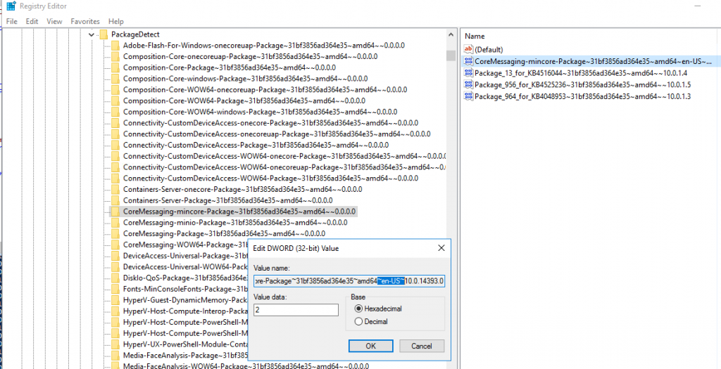
My day to day involves a good deal of sysadmin work, mostly Windows networks for small business customers. I ran into the above error on a Dell Server 2016 machine when trying to uninstall Windows components (Hyper-V in this case). This post gave me hint I needed to figure out the root cause, some missing language packs.
Now the original post recommends reinstalling the OS, which is a huge non-starter for me in an environment with a single file/AD server. The long fix starts with uninstalling language packs using the lpksetup tool and then manually removing references to any missing packs under the HKEY_LOCAL_MACHINE\SOFTWARE\Microsoft\Windows\CurrentVersion\Component Based Servicing\PackageDetectregistry subkeys. There are lots of them, literally thousands.
Just one of the 7600 registry values that need to be filtered.
I really needed to resolve this, so I spent an hour writing a PowerShell script to run through each subkey value and remove the one’s that referenced a missing language pack. In my case it was a German edition, so we’re searching for the string ‘~de-DE~’ below:
It’s pretty simple, but was frustrating because of the need to get the .psobject.properties. I went through a lot of iterative testing to make sure that I targeted the proper values. Hopefully this helps someone else avoid a reinstallation. After running this script I was able to remove the Windows Hyper-V feature with no problems. I assume that this error was caused by an aborted uninstallation of one of the language packs. I’m not sure how they got on there, but assume that it was a Dell image load or something.
I’ve settled into a bit of a rhythm lately, spending my days working on Python code from home, continuing my project to integrate the various vendor that I use as part of my job via their APIs. In the evenings, after the girls have gone to bed, I’ve been working on various personal and school projects, or watching various computer science related videos. Friday to Saturday evenings, however, we’ve been doing a tech Shabbat, so I’ve been trying to find ways to get the girls out of the house as much as possible. More on that another time.
I finished watching the MIT Lisp series a week or two ago. It’s hard to believe that it’s a freshman-level class, as it’s fair to say that it’s probably more challenging than anything I’ve taken at my current university other than autotonoma theory. It covers so much, and Lisp, or Scheme, rather, has such a simple syntax, that it is really interesting to see how everything can be built up from these simple data structures and procedures.
Since I finished those, I’ve been watching a lot of Pycon videos to try and level up my understanding of some of the more advanced programming idioms that Python has. I’ve finally wrapped my head around list and dictionary comprehension, and have finally figured out what generators are good for. I’m going to to be exploring async and threading next.
In the last post, I was talking about the Ameritrade API and the work I’ve been doing to wrap my head around that. Well, yesterday I logged into my account and saw a notice that they were being bought out by Charles Schwab. Since I’ve been rather frustrated with the whole debugging process for that, I’ve decided to step away from that for a few days and decide whether it makes sense to continue with that or not. I don’t get the sense hat Schwab has a a very open system, and I’m not really enthusiastic about starting from scratch. Maybe I can find a broker with an open, standards compliant API that I can rollover to?
One of the main vendors that we use at work has a SOAP API that uses XML to transmit data. I spent several days trying to figure out how all the WSDL definitions work to see if I could use some metaprogramming to dynamically inspect the various entity attributes. Creating XML queries via chained method calls seems overly complicated, so I’ve been looking at how Django builds their SQL queries using QuerySet calls like Entity.objects.get(id='foo'). It’s much simpler, but it’s such a higher-level design program that I’ve become overwhelmed.
In general, that’s been the feeling lately, overwhelmed. It’s a different type of feeling than I have when I’m overcome with personal obligations and scheduling items. Now, it’s more like my programming ideas are getting to the point where it’s getting hard to intellectually manage them. The solution at this point seems to be to step back and work on something else, and give my brain time to work on the problem offline. An idea might pop into my head on it’s own, or a programming video might give me an idea on how to tackle a problem.
I’ve been trying to stay focused, by limiting the number of things that I’m allowing myself to work on, whether software projects or learning a new piano piece. But sometime you have to step back, and apply skills in to other problems that may reveal solutions in unexpected ways.
My life goal of automating my job out of existence continues unabated. I’ve been spending a lot of time dealing with the APIs of the various vendors that we deal with, and I’ve spent a lot of time pouring over JSON responses. Most of these are multi-level structures, and usually leads to some clunky accessor code like object['element']['element']. I much rather prefer the more elegant dot notation of object.element.element instead, but getting from JSON to objects hasn’t been something I’ve wanted to spend much time on. Sure, there are a few options to do this using standard Python, but QuickType is by far the best solution out there.
I’ve been using the web-based version for the past few days to create an object library for Ameritrade’s API. Now first off, I’m probably going overboard and violating YAGNI (you ain’t gonna need it) principles by trying to include everthing that the API can return, but it’s been a good excuse to learn more about JSON schemas.
JSON schema with resultant Python code on right.
One of the things that I wish I’d caught earlier is that the recommended workflow in Quicktype is to start with example JSON data, and convert it to a JSON schema before going from that schema to your target language. I’d been trying to go straight from JSON to Python, and there were some problems. First off, the Ameritrade schema has a lot more types than I’ll need: there are two subclasses of securities account, and 5 different ones for the various instrument class. I only need a small subset of that, but thankfully Quicktype automatically combines these together. Secondly, Ameritrade’s response summary, both the schema and the JSON examples, aren’t grouped together in a way that can be parsed efficiently. I spent countless hours trying to combine things into a schema that is properly referenced and would compile properly.
But boy, once it did. Quicktype does a great job of generating code that can process JSON into a Python object. There are handlers for all of the various data types, and Quicktype will actually type check everything from ints to lists, dicts to unions (for handling Nones), and will process classes back out to JSON as well. Subobject parsing works very well. And even if you don’t do Python, it has a an impressive number of languages that it outputs to.
One problem stemming from my decision to use Ameritrade’s response summary JSON code instead of their schema is that the example code uses 0 instead of 0.0 where a float would be applicable. This led to Quicktype generating it’s own schema using integers instead of the JSON schema float equivalent, number. Additionally, Ameritrade doesn’t designate any properties as required, whereas Quicktype assumes everything in your example JSON is, which has led to a lot of failed tests.
Next, I’ll likely figure out how to run Quicktype locally via CLI and figure out some sort of build process to use to keep my object code in sync with my schema definitions. There’s been a lot of copypasta going on the past few days, and having it auto update and run tests when the schema changes seems like a good pipeline opportunity. I’ve also got to spend some more time understanding how to tie together complex schema. Ameritrade’s documentation isn’t up to standard, so figuring out to break them up into separate JSON objects and reference them efficiently will be crucial if I’m going to finish converting the endpoints that I need for my project.
That said, Quicktype is a phenomenal tool, and one that I am probably going to use for other projects that interface with REST APIs.
Three Years of Misery Inside Silicon Valley’s Happiest Company, by Nitasha Tiku:The cover story of this month’s issue a really in-depth piece about the chaos that has been plaguing of the eponymous internet search company, Google. One of the things I love about Wired is their long form reporting, and this article is several thousand words, about 14 pages of text in nine parts. Tiku details the leaks from inside the company that seemingly destroyed the company’s unspoken rule of ‘what happens at Google, stays in Google’. Social justice activists tore down the company’s missteps with regard to sexual harrassment by managers and execs, betraying their “don’t do evil” motto, through dealings with authoritarian China and the United States military.
The article really opens up a look at the inner culture of Google, how they had a fairly open culture, with C-level executives making themselves open for questioning from staffers, and with rank-and-file employees creating sub-cultures within the company. T
The story starts in January 2017, as employees took to the streets after the Trump administration’s travel ban was declared. The company stood behind their employees and stood up for immigrant rights. Then in June, an engineer named James Damore release a 10-page memo ‘explaining’ why there weren’t more female engineers in the industry. Damore was reacting to efforts to promote female engineers within the company, and claimed that this was a bad idea since there were biological reasons why there aren’t more women in STEM fields.
The eventual backlash to Damore’s memo, and his eventual dismissal, started a culture war between the company’s conservatives. Apparently, this minority within Google had been existing within their own corner of the company, but following this, some of them became emboldened and began to step up their opposition and trollishness. They doxed several of the liberal organizers, thereby breaking the company’s sacred rule of non-disclosure.
This episode is just one of several that Tiku details. By the end of the piece, it’s clear that Google’s culture has been transformed, and that while their employees may still be sticking to their ‘don’t be evil’ motto, the executives of the company, driven by shareholder capitalist growth demands, have lost their way.
FAN-tastic Planet: When I was a teenager, growing up in the mid 90’s, Wired was the coolest magazine on the planet. I felt that it offered up both a vision of the future and secret knowledge about where things were headed. Wired was an essential fuel for the ideas that eventually led to my career in computers and programming. Now, having learned more about the nascent cyberpunk culture that Wired killed off in favor off Dot Com boom and bust, that I wonder more about what could have been. I bring this up because I was almost shocked to read the intro to this special culture section in this issue.
“A person sitting at a computer – it was a mystical sight. Once,” it opens, before going further into something straight out of a Rushkoff monologue: “The users, we humans were the almight creator-gods of the dawning digial age, and the computers did our bidding. We were in charge. In today’s world, subject and object have switched places… Computers run the show now, and we -mere data subjects.” It’s almost like they literally took Rushkoff’s point about ‘figure and ground’ verbatim. Please forgive me, dear reader, for mistaking if his point isn’t original. But given his disdain for Wired’s entire raison d’etre during the 90’s and aughts, I find it entirely ironic that they have this section: fan-fic-writing nerds; Netflix’s turn toward Choose-Your-Own-Adventure-style programming; social-media influencers ‘connecting’ with fans over special, subscriber only feeds; and the rise of a new generation of crossword-puzzle writers who are bringing new, diverse voices to another field traditionally dominated by white men. (This last one actually includes a crossword, and let to several days of puzzling on my part.)
Free Riders, by Zeynep Tufekci: The front pages of this issue have the standard Wired fare, gadgets and the latest tech. This time it’s smart-writing tools and augmented-reality gizmos. A bit about the current NASA Mars rover being built, another extolling the joys of world-building video games, another bemoaning Facebook’s creepy dating feature. I wanted to end with a mention of Tufekci’s bit about the prevalence of commercial companies that are built on top of the free, open source tools that have been released to the internet. Not that this is a problem, per se, but there have been many instances of packages that have been so instrumental to the success of these companies, and to the industry in general, that have had security issues, or depended on the unpaid efforts of some very overworked contributors. Tufekci details two pertinent examples: the Heartbleed bug, which affected the OpenSSL spec used to protect almost all web traffic, and core-js, a Javascript library widely used in web browsers.
In the latter case, the developer had been working on the library almost every day for five years without pay, and had solicited less than a hundred dollars. While some might blame him for not taking advantage of his project’s popularity and using it to leverage himself into a high-paying gig somewhere, the issue highlights a problem with the web’s altruistic origins, that have long since been abused by corporation. At least, in the case of OpenSSL, they were able to guilt some firms into providing more funding, but we’ve got a long way to figure out a way to reward these open source programmers that have provided the tools that the web is built on.
In our previous posts (part 1, part 2) we showed how to get historical stock data from the Alpha Vantage API, use Pickle to cache it, and how prep it in Pandas. Now we are ready to throw it in Prophet!
So, after loading our main.py file, we get ticker data by passing the stock symbol to our get_symbol function, which will check the cache and get daily data going back as far as is available via AlphaVantage.
>>> symbol = "ARKK"
>>> ticker = get_symbol(symbol)
./cache/ARKK_2019_10_19.pickle not found
{'1. Information': 'Daily Prices (open, high, low, close) and Volumes', '2. Symbol': 'ARKK', '3. Last Refreshed': '2019-10-18', '4. Output Size': 'Full size', '5. Time Zone': 'US/Eastern'}
{'1: Symbol': 'ARKK', '2: Indicator': 'Simple Moving Average (SMA)', '3: Last Refreshed': '2019-10-18', '4: Interval': 'daily', '5: Time Period': 60, '6: Series Type': 'close', '7: Time Zone': 'US/Eastern'}
{'1: Symbol': 'ARKK', '2: Indicator': 'Relative Strength Index (RSI)', '3: Last Refreshed': '2019-10-18', '4: Interval': 'daily', '5: Time Period': 60, '6: Series Type': 'close', '7: Time Zone': 'US/Eastern Time'}
./cache/ARKK_2019_10_19.pickle saved
Running Prophet
Now we’re not going to do anything here with the original code other than wrap it in a function that we can call again later. Our alpha_df_to_prophet_df() function renames our datetime index and close price series data columns to the columns that Prophet expects. You can follow the original Medium post for an explanation of what’s going on; we just want the fitted history and forecast dataframes in our return statement.
The whole process runs within a minute. Even twenty years of Google daily data can be processed quickly.
The last thing we want to do is concat the forecast data back to the original ticker data and Pickle it back to our file system. We rename our index back ‘date’ as it was before we modified it, then join it to the original Alpha Vantage data.
def concat(ticker, df_forecast):
    df = df_forecast.rename(columns={'ds': 'date'}).set_index('date')[['trend', 'yhat_lower', 'yhat_upper', 'yhat']]
    frames = [ticker, df]
    result = pd.concat(frames, axis=1)
    return result
Seeing the results
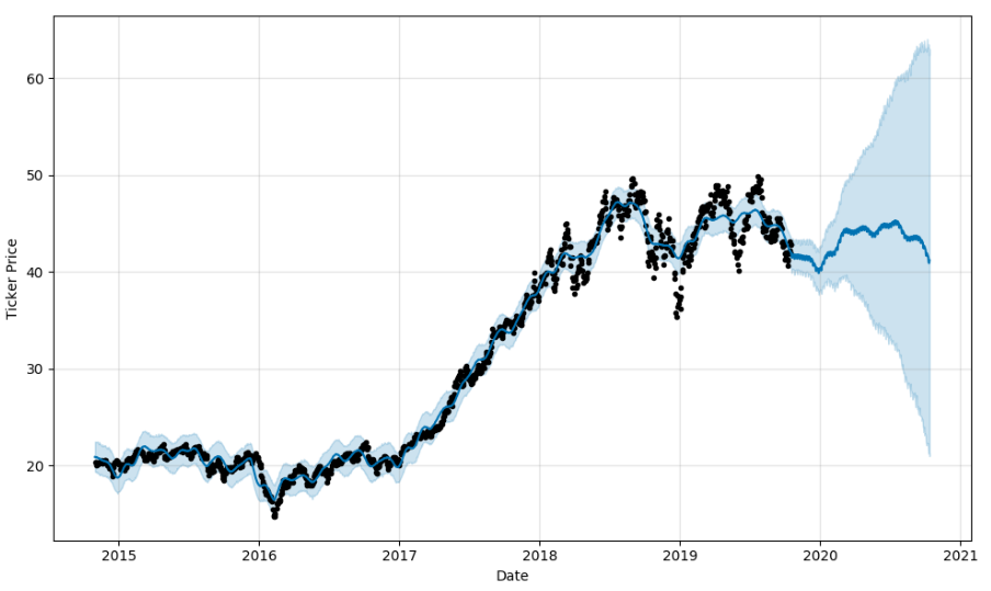
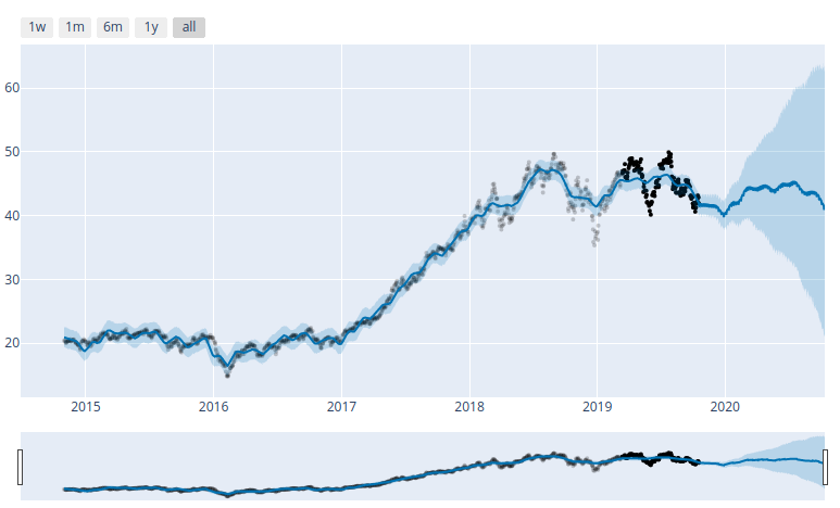
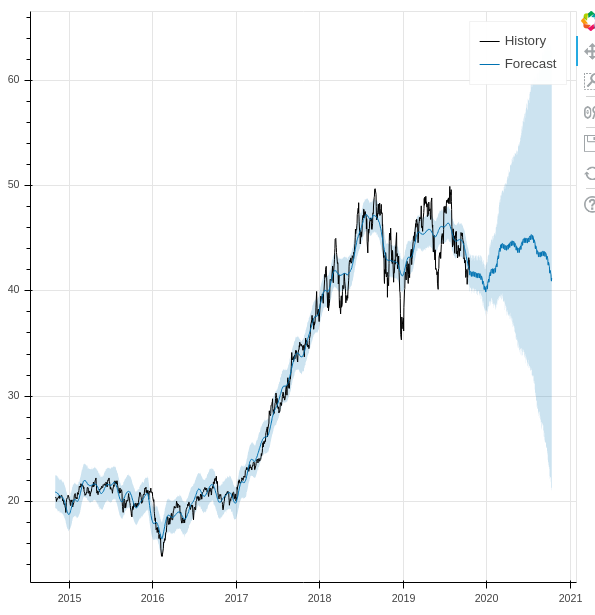
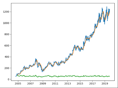
Since these are Pandas dataframes, we can use matplotlib to see the results, and Prophet also includes Plotly support. But as someone who looks at live charts in TradingView throughout the day, I’d like something more responsive. So we loaded the Bokeh library and created the following function to match.
ARKK plot using matplotlib. Static only. ARKK plot in Plotly. Not great. UI is clunky and doesn’t work well in my dev VM browser.
ARKK plot in Bokeh. Can easily zoom and pan. Lovely.
Putting it all together
Our ultimate goal here is to be able to process large batches of stocks, downloading the data from AV and processing it in Prophet in one go. For our initial run, we decided to start with the bundle of stocks in the ARK Innovation ETF. So we copied the holdings into a Python list, and created a couple of functions. One to process an individual stock, an another to process the list. Everything in the first function should be familiar except for two things. One, we added a check for the ‘yhat’ column to make sure that we didn’t inadvertently reprocess any individual stocks while we were debugging. We also refactored get_filename, which just adds the stock ticker plus today’s date to a string. It’s used in get_symbol during the Alpha Vantage call, as well as here when we save the Prophet-ized data back to the cache.
Finally, our process_list function. We had a bit of a wrinkle at first. Since we’re using the free AlphaVantage API, we’re limited to 5 API calls per minute. Now since we’re making three in each get_symbol() call we get an exception if we process the loop more than once in sixty seconds. Now I could have just gotten rid of the SMA and RSI calls, ultimately decided just to calculate the duration of each loop and just sleep until the minute was up. Obviously not the most elegant solution, but it works.
def process_list(symbol_list):
    for symbol in symbol_list:
        start = time.time()
        process(symbol)
        end = time.time()
        elapsed = end - start
        print ("Finished processing {} in {}".format(symbol, elapsed))
        if elapsed > 60:
            continue
        elif elapsed < 1:
            continue
        else:
            print('Waiting...')
            time.sleep(60 - elapsed)
            continue
So from there we just pass our list of ARKK stocks, go for a bio-break, and when we come back we’ve got a cache of Pickled Pandas data and Bokeh plots for about thirty stocks.
Where do we go now
Now I’m not putting too much faith into the results of the Prophet data, we didn’t do any customizations, and we just wanted to see what we can do with it. In the days since I started writing up this series, I’ve been thinking about ways to calculate the winners of the plots via a function call. So far I’ve come up with this discount function, that determines the discount of the current price of an asset relative to Prophet’s yhat prediction band.
A negative number for the discount indicates that the current price is below the prediction band, and may be a buy. Likewise, anything over 100 is above the prediction range and is overpriced, according to the model. We did ultimately pick two out of the ARKK holding that were well below the prediction range and showed a long term forecast, and we’ve started scaling in modestly while we see how things play out.
If we were more cautious, we’d do more backtesting, running limited time slices through Prophet and comparing forecast accuracy against the historical data. Additionally, we’d like to figure out a way to weigh our discount calculation against the accuracy projections.
There’s much more to to explore off of the original Medium post. We haven’t even gotten into integrating Alpha Vantage’s cryptoasset calls, nor have we done any of the validation and performance metrics that are part of the tutorial. It’s likely a part 4 and 5 of this series could follow. Ultimately though, our interest is to get into actual machine learning models such as TensorFlow and see what we can come up with there. While we understand the danger or placing too much weight into trained models, I do think that there may be value to using these frameworks as screeners. Coupled with the value averaging algorithm that we discussed here previously, we may have a good strategy for long-term investing. And anything that I can quantify and remove the emotional factor from is good as well.
I’ve learned so much doing this small project. I’m not sure how much more we’ll do with Prophet per se, but the Alpha Vantage API is very useful, and I’m guessing that I’ll be doing a lot more with Bokeh in the future. During the last week I’ve also discovered a new Python project that aims to provide a unified framework for coupling various equity and crypto exchange APIs with pluggable ML components, and use them to execute various trading strategies. Watch this space for discussion on that soon.
Facebook’s Prophet module is a trend forecasting library for Python. We spent some time over the last week going over it via this awesome introduction on Medium, but decided to do some refactoring to make it more reusable. Previously, we setup our pipenv virtual environment, separated sensitive data from our source code using dotenv, and started working with Alpha Vantage’s stock price and technical indicator API. In this post we’ll save our fetched data using Pickle and do some dataframe manipulations in Pandas. Part 3 is also available now.
Pickling our API results
When we left off, we had just wrote our get_time_series function, to which we pass 'get_daily' or such and a symbol for the stock that we would like to retrieve. We also have our get_technical function that we can use to pull any of the dozens of indicators available through Alpha Vantage’s API. Following the author’s original example, we can load Apple’s price history, simple moving average and RSI using the following calls:
symbol = 'AAPL'
ticker = get_time_series('get_daily', symbol, outputsize='full')
sma = get_technical('get_sma', symbol, time_period=60)
rsi = get_technical('get_rsi', symbol, time_period=60)
We’ve now got three dataframes. In the original piece, the author shows how you can export and import this dataframe using Panda’s .to_csv and read_csv functions. Saving the data is a good idea, especially during this stage of development, because it allows us to cache out data and reduce the number of API calls. (Alpha Vantage’s free tier allows 5 calls per minute, 500 a day. ) However, using CSV to save Panda’s dataframes is not recommended, as you will use index and column data. Python’s Pickle module will serialize the data and preserve it whole.
For our implementation, we will create a get_symbol function, which will check a local cache folder for a copy of the ticker data and load it. Our file naming convention uses the symbol string plus today’s date. Additionally, we concat our three dataframes into one using Pandas concat function:
def get_symbol(symbol):
    CACHE_DIR = './cache'
    # check if cache exists
    symbol = symbol.upper()
    today = datetime.now().strftime("%Y_%m_%d")

    file = CACHE_DIR + '/' + symbol + '_' + today + '.pickle'
    if os.path.isfile(file):
        # load pickle
        print("{} Found".format(file))
        result = pickle.load(open(file, "rb"))
    else:
        # get data, save to pickle
        print("{} not found".format(file))
        ticker = get_time_series('get_daily', symbol, outputsize='full')
        sma = get_technical('get_sma', symbol, time_period=60)
        rsi = get_technical('get_rsi', symbol, time_period=60)

        frames = [ticker, sma, rsi]
        result = pd.concat(frames, axis=1)
        pickle.dump(result, open(file, "wb"))
        print("{} saved".format(file))
    return result
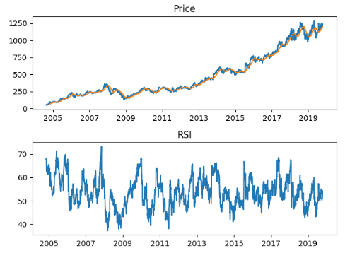
Charts!
The original author left out all his chart code, so I had to figure things out on my own. No worries.
We saved both of these in a plot_ticker function for reuse in our library. Now I am no expert on matplotlib, and have only done some basic stuff with Plotly in the past. I’m probably spoiled by looking at TradingView’s wonderful chart tools and dynamic interface, so being able to drag and zoom around in the results is really important to me from a usability standpoint.
Now I am no expert on matplotlib, and have only done some basic stuff with Plotly in the past. I’m probably spoiled by looking at TradingView’s wonderful chart tools and dynamic interface, so being able to drag and zoom around in the results is really important to me from a usability standpoint. So we’ll leave matplotlib behind from here, and I’ll show you how I used Bokeh in the next part.
Framing our data
We already showed how we concat our price, SMA and RSI data together earlier. Let’s take a look at our dataframe metadata. I want to show you the columns, the dtype of those columns, as well as that of the index. Tail is included just for illustration.
>>> ticker.columns
Index(['1. open', '2. high', '3. low', '4. close', '5. volume', 'SMA', 'RSI'], dtype='object')

>>> ticker.dtypes
1. open      float64
2. high      float64
3. low       float64
4. close     float64
5. volume    float64
SMA          float64
RSI          float64
dtype: object

>>> ticker.index
DatetimeIndex(['1999-10-18', '1999-10-19', '1999-10-20', '1999-10-21',
               '1999-10-22', '1999-10-25', '1999-10-26', '1999-10-27',
               '1999-10-28', '1999-10-29',

>>> ticker.tail()
            1. open  2. high  3. low  4. close   5. volume       SMA      RSI
date
2019-10-09   227.03   227.79  225.64    227.03  18692600.0  212.0238  56.9637
2019-10-10   227.93   230.44  227.30    230.09  28253400.0  212.4695  57.8109
Now we don’t need all this for Prophet. In fact, it only looks at two series, a datetime column, labeled ‘ds’, and the series data that you want to forecast, a float, as ‘y’. In the original example, the author renames and recasts the data, but this is likely because of the metadata loss when importing from CSV, and isn’t strictly needed. Additionally, we’d like to preserve our original dataframe as we test our procedure code, so we’ll pass a copy.
In the first line of prophet_df =we’re selecting only the ‘close’ price column, which is returned with the original DateTimeIndex. We reset the index, which makes this into a ‘date’ column. Finally we rename them accordingly.
And that’s it for today! Next time we will be ready to take a look at Prophet. We’ll process our data, use Bokeh to display it, and finally write a procedure which we can use to process data in bulk.
I’ve spent countless hours this past week working with Facebook’s forecasting library, Prophet. I’ve seen lots of crypto and stock price forecasting and prediction model tutorials on Medium over the past few months, but this one by Senthil E. focusing on Apple and Bitcoin prices got my attention, and I just finished putting together a Python file that takes his code and builds it into some reusable code.
Now after getting to know it better, I can say that it’s not the most sophisticated package out there. I don’t think it was intended for forecasting stock data, but it is fast and allows one to see trends. Plus I learned a lot using it, and had fun. So what more can you ask for?
As background, I’ve been working on refining the Value Averaging functions I wrote about last week and had been having some issues with the Pandas Datareader library’s integration with the Alpha Vantage stock history API. Senthil uses a different third-party module that doesn’t have any problems, so that was good.
Getting started
I ran into some dependency hell during my initial setup. I spawned a new pipenv virtual environment and installed Jupyter notebook, but a prompt-toolkit conflict led to some wasted time. I started by copying the original code into a notebook, and go that running first. I quickly started running into problems with the author’s code.
I did get frustrated at one point and setup Anaconda in a Docker container on another machine, but I was able to get my main development machine up and running. We’ll save Conda for another day!
Importing the libraries
Like most data science projects, this one relies on Pandas and matplotlib, and the Prophet library has some Plotly integration. The author had the unused wordcloud package in his code for some reason as well, and it’s not entirely certain how he’s using the seaborn module, since he doesn’t explain his plots. He also listed two different Alpha Vantage modules despite only using one. I believe he may have put the alphaVantageAPI module in first before switching to the more useable alpha_vantage one.
We eventually added pickle, dotenv, and bokeh modules, as we’ll see shortly, as well as os, time, datetime.
import os
import pickle
import time
from datetime import datetime
import pandas as pd
from fbprophet import Prophet
from fbprophet.plot import plot_plotly
from bokeh.plotting import figure, output_file, show, save

import matplotlib.pyplot as plt
# import plotly.offline as py
# import numpy as np
# import seaborn as sns
# from alphaVantageAPI.alphavantage import AlphaVantage

from alpha_vantage.timeseries import TimeSeries
from alpha_vantage.techindicators import TechIndicators
from dotenv import load_dotenv
Protect your keys!
One of the first modules that we add to every project nowadays is python-dotenv. I’ve really been trying to get disciplined about 12-factor applications, and since I’m committing all of my projects to Gitlab these days, I can be sure not to commit my API keys to a repo or post them in a gist on my blog!
Also, pipenv shell automatically loads .env files, which is another reason why you should be using them.
If there is anything I hate, it’s repeating myself, or having to use the same block of code several times within a document. Now I don’t know whether the author kept the following two blocks of code in his story for illustrative purposes, or if this is just how he had it loaded in his notebook, but it gave me a complex.
from alpha_vantage.techindicators import TechIndicators
import matplotlib.pyplot as plt
ti = TechIndicators(key='<YES, he left his API KEY here!>',output_format='pandas')
data, meta_data = ti.get_sma(symbol='AAPL',interval='daily', time_period=60,series_type = 'close')
data.plot()
plt.show()

from alpha_vantage.techindicators import TechIndicators
import matplotlib.pyplot as plt
ti = TechIndicators(key='Youraccesskey',output_format='pandas')
data, meta_data = ti.get_rsi(symbol='AAPL',interval='daily', time_period=60,series_type = 'close')
data.plot()
plt.show()
If you look at the Alpha Vantage API documentation, there are separate endpoints for the time series and technical endpoints. The time series endpoint has different function calls for daily, weekly, monthly, &c.., and the Python module we’re using has separate methods for each. Same for the technical indicators. Now in the past, when I’ve tried to wrap APIs I would have had separate calls for each function, but I learned something about encapsulation lately and wanted to give something different a try.
Since the technical indicators functions share the same set of positional arguments, we can create a wrapper function where we pass the the name of the function (the indicator itself) that we want to get, the associated symbol, as well as any keyword arguments that we want to specify. We use the getattr method to find the class’s function by name, and pass on our variables using **kwargs.
def get_technical(indicator, symbol, **kwargs):
    function = getattr(ti, indicator)
    data, meta_data = function(symbol=symbol, **kwargs)
    print(meta_data)
    return data

sma = get_technical('get_sma', symbol, time_period=60)
rsi = get_technical('get_rsi', symbol, time_period=60)
Since most of the kwargs in the original were redundant, we only need to pass what we want to override. We’ve not really reduced the original code, to be honest, but we can customize what happens after in a way that we can be consistent, without having to write multiple functions for each function in the original module. Additionally, we can do this for the time series functions as well.
# BEFORE
from alpha_vantage.timeseries import TimeSeries
import matplotlib.pyplot as plt
ts = TimeSeries(key='Your Access Key',output_format='pandas')
apple, meta_data = ts.get_daily(symbol='AAPL',outputsize='full')
apple.head()

#AFTER
def get_time_series(time_series, symbol, **kwargs):
    function = getattr(ts, time_series)
    data, meta_data = function(symbol=symbol, **kwargs)
    print(meta_data)
    return data

ticker = get_time_series('get_daily', symbol, outputsize='full')
You can see that both functions are almost identical, except that the getattr call is passing the ts and ti classes. Ultimately, I’ll extend this to the cryptocurrencies endpoint as well, and be able to add any exception checking and debugging that I need for the entire module, and use one function for all of it.
Writing this code was one of those level-up moments when I got an idea and knew that I ultimately understood programming at an entirely different level than I had a few months ago.
Next, we’ll use Pickle to save and load our data, and start manipulating our dataframes before passing them to Prophet. Read part two.